To Create Heat Map in excel follow these steps:
Wednesday, October 21, 2015

Wednesday, October 9, 2013
Sequentially numbering multiple copies of single document using a macro
Create a bookmark named “SerialNumber” in the document where you want the Serial Number to appear. It can be in the header or footer if that is
where you want the number.
Then create a macro containing the following commands to print the document.
It will ask for the number of copies that you want to make and sequentially number each copy.
The first time this macro runs, the first copy will be numbered 1 and when it finishes running, it will store in aSettings.Txt file the number that is one more that the number on the last copy.
The next time the macro is run, it will start numbering the copies from that number. If when you first start, you want the numbers to start at some number other than 1, run the macro, entering 1 as the number of copies and then open Settings.Txt file and replace the number in the file with the number that you want as the first in the series.
At any time thereafter, if you want the series to start at a particular number, you can open that file and replace the number in it with the number that you want to be the first in the series.
Then create a macro containing the following commands to print the document.
It will ask for the number of copies that you want to make and sequentially number each copy.
The first time this macro runs, the first copy will be numbered 1 and when it finishes running, it will store in aSettings.Txt file the number that is one more that the number on the last copy.
The next time the macro is run, it will start numbering the copies from that number. If when you first start, you want the numbers to start at some number other than 1, run the macro, entering 1 as the number of copies and then open Settings.Txt file and replace the number in the file with the number that you want as the first in the series.
At any time thereafter, if you want the series to start at a particular number, you can open that file and replace the number in it with the number that you want to be the first in the series.
Dim Message As String, Title As
String, Default As String, NumCopies As Long
Dim Rng1 As Range
' Set prompt.
Message = "Enter the number of copies that you want to print"
' Set title.
Title = "Print"
' Set default.
Default = "1"
' Display message, title, and default value.
NumCopies = Val(InputBox(Message, Title, Default))
SerialNumber = System.PrivateProfileString("C:\Settings.Txt", _
"MacroSettings", "SerialNumber")
If SerialNumber = "" Then
SerialNumber = 1
End If
Set Rng1 = ActiveDocument.Bookmarks("SerialNumber").Range
Counter = 0
While Counter < NumCopies
Rng1.Delete
Rng1.Text = SerialNumber
ActiveDocument.PrintOut
SerialNumber = SerialNumber + 1
Counter = Counter + 1
Wend
'Save the next number back to the Settings.txt file ready for the next use.
System.PrivateProfileString("C:\Settings.txt", "MacroSettings", _
"SerialNumber") = SerialNumber
'Recreate the bookmark ready for the next use.
With ActiveDocument.Bookmarks
.Add Name:="SerialNumber", Range:=Rng1
End With
ActiveDocument.Save
If you want the Serial Number to appear in a particular format, e.g. 001, 002, etc, replace the line
Dim Rng1 As Range
' Set prompt.
Message = "Enter the number of copies that you want to print"
' Set title.
Title = "Print"
' Set default.
Default = "1"
' Display message, title, and default value.
NumCopies = Val(InputBox(Message, Title, Default))
SerialNumber = System.PrivateProfileString("C:\Settings.Txt", _
"MacroSettings", "SerialNumber")
If SerialNumber = "" Then
SerialNumber = 1
End If
Set Rng1 = ActiveDocument.Bookmarks("SerialNumber").Range
Counter = 0
While Counter < NumCopies
Rng1.Delete
Rng1.Text = SerialNumber
ActiveDocument.PrintOut
SerialNumber = SerialNumber + 1
Counter = Counter + 1
Wend
'Save the next number back to the Settings.txt file ready for the next use.
System.PrivateProfileString("C:\Settings.txt", "MacroSettings", _
"SerialNumber") = SerialNumber
'Recreate the bookmark ready for the next use.
With ActiveDocument.Bookmarks
.Add Name:="SerialNumber", Range:=Rng1
End With
ActiveDocument.Save
Rng1.Text = SerialNumber
with
Rng1.Text = Format(SerialNumber, "00#")
Tuesday, October 8, 2013
To run a macro at schedule time
If you want to keep your workbook open and run code at a specified time, later on, then try this..
Insert a new code module to your project -or- use one that you already have in your project.
Create a scheduler subroutine as shown below:
Create a subroutine (or function) that you want to run. Here is one for this example:
You could probably pass the time value you want the Scheduler() sub to execute your sub(s) or function(s) in as a parameter in the sub.
You could probably run a sub 5 hours from now, lets say. I.E. Application.OnTime Now + TimeValue("05:00:00"), "TheScheduledSub"
Insert a new code module to your project -or- use one that you already have in your project.
Create a scheduler subroutine as shown below:
Sub Scheduler()

'-- RUNS SUB(S) (OR FUNCTIONS) AT TIME SCHEDULED.

    Application.OnTime TimeValue("11:46:40"), "TheScheduledSub"

End Sub
Create a subroutine (or function) that you want to run. Here is one for this example:
Sub TheScheduledSub()

    Debug.Print "TheScheduledSub() has run at " & Time

End Sub
Scheduler() will execute TheScheduledSub() at the exact time specified inside Scheduler(), defined by TimeValue. You can read more about TimeValue here.You could probably pass the time value you want the Scheduler() sub to execute your sub(s) or function(s) in as a parameter in the sub.
You could probably run a sub 5 hours from now, lets say. I.E. Application.OnTime Now + TimeValue("05:00:00"), "TheScheduledSub"
Thursday, September 5, 2013
Convert DD/MM/YYYY format to MM/DD/YYYY format and vice versa
Here is the solution to convert any data format to your required format
For Example:
DD/MM/YYYY to MM/DD/YYYY
MM/DD/YYYY to DD/MM/YYYY
also to
YYYY/MM/DD
MM/YYYY/DD
DD/YYYY/MM
YYYY/DD/MMMM
Follow this method to do that:
Select Dates
Data Menu
Text To Column
Delimited - Untick all options (Can also use Fixed Width)
Next
Select Date Option
Finish
For Example:
DD/MM/YYYY to MM/DD/YYYY
MM/DD/YYYY to DD/MM/YYYY
also to
YYYY/MM/DD
MM/YYYY/DD
DD/YYYY/MM
YYYY/DD/MMMM
Follow this method to do that:
Select Dates
Data Menu
Text To Column
Delimited - Untick all options (Can also use Fixed Width)
Next
Select Date Option
Finish
Wednesday, September 4, 2013
Copy all mail contents from Outlook to excel sheets separate by each Column
To copy all the mail contents from outlook to excel in separate column, please do the following:
The Macro code is:
Sub CopyToExcel()
Dim xlApp As Object
Dim xlWB As Object
Dim xlSheet As Object
Dim olItem As Outlook.MailItem
Dim vText As Variant
Dim sText As String
Dim vItem As Variant
Dim i As Long
Dim rCount As Long
Dim bXStarted As Boolean
Const strPath As String = "C:\Sample.xlsx" 'the path of the workbook
If Application.ActiveExplorer.Selection.Count = 0 Then
MsgBox "No Items selected!", vbCritical, "Error"
Exit Sub
End If
On Error Resume Next
Set xlApp = GetObject(, "Excel.Application")
If Err <> 0 Then
Application.StatusBar = "Please wait while Excel source is opened ... "
Set xlApp = CreateObject("Excel.Application")
bXStarted = True
End If
On Error GoTo 0
'Open the workbook to input the data
Set xlWB = xlApp.Workbooks.Open(strPath)
Set xlSheet = xlWB.Sheets("Sheet1")
rCount = xlSheet.UsedRange.Rows.Count
'Process each selected record
For Each olItem In Application.ActiveExplorer.Selection
sText = olItem.Body
vText = Split(sText, Chr(13))
'Find the next empty line of the worksheet
rCount = rCount + 1
'Check each line of text in the message body
For i = UBound(vText) To 0 Step -1
If InStr(1, vText(i), "Name:") > 0 Then
vItem = Split(vText(i), Chr(58))
xlSheet.Range("A" & rCount) = Trim(vItem(1))
End If
If InStr(1, vText(i), "Email:") > 0 Then
vItem = Split(vText(i), Chr(58))
xlSheet.Range("B" & rCount) = Trim(vItem(1))
End If
If InStr(1, vText(i), "Phone:") > 0 Then
vItem = Split(vText(i), Chr(58))
xlSheet.Range("C" & rCount) = Trim(vItem(1))
End If
If InStr(1, vText(i), "Address:") > 0 Then
vItem = Split(vText(i), Chr(58))
xlSheet.Range("D" & rCount) = Trim(vItem(1))
End If
If InStr(1, vText(i), "Event:") > 0 Then
vItem = Split(vText(i), Chr(58))
xlSheet.Range("E" & rCount) = Trim(vItem(1))
End If
If InStr(1, vText(i), "Location:") > 0 Then
vItem = Split(vText(i), Chr(58))
xlSheet.Range("F" & rCount) = Trim(vItem(1))
End If
Next i
xlWB.Save
Next olItem
xlWB.Close SaveChanges:=True
If bXStarted Then
xlApp.Quit
End If
Set xlApp = Nothing
Set xlWB = Nothing
Set xlSheet = Nothing
Set olItem = Nothing
End Sub
- Copy the below code in outlook
- Crate a file in C folder
- run the macro from Outlook
- Results will be in excel
The Macro code is:
Sub CopyToExcel()
Dim xlApp As Object
Dim xlWB As Object
Dim xlSheet As Object
Dim olItem As Outlook.MailItem
Dim vText As Variant
Dim sText As String
Dim vItem As Variant
Dim i As Long
Dim rCount As Long
Dim bXStarted As Boolean
Const strPath As String = "C:\Sample.xlsx" 'the path of the workbook
If Application.ActiveExplorer.Selection.Count = 0 Then
MsgBox "No Items selected!", vbCritical, "Error"
Exit Sub
End If
On Error Resume Next
Set xlApp = GetObject(, "Excel.Application")
If Err <> 0 Then
Application.StatusBar = "Please wait while Excel source is opened ... "
Set xlApp = CreateObject("Excel.Application")
bXStarted = True
End If
On Error GoTo 0
'Open the workbook to input the data
Set xlWB = xlApp.Workbooks.Open(strPath)
Set xlSheet = xlWB.Sheets("Sheet1")
rCount = xlSheet.UsedRange.Rows.Count
'Process each selected record
For Each olItem In Application.ActiveExplorer.Selection
sText = olItem.Body
vText = Split(sText, Chr(13))
'Find the next empty line of the worksheet
rCount = rCount + 1
'Check each line of text in the message body
For i = UBound(vText) To 0 Step -1
If InStr(1, vText(i), "Name:") > 0 Then
vItem = Split(vText(i), Chr(58))
xlSheet.Range("A" & rCount) = Trim(vItem(1))
End If
If InStr(1, vText(i), "Email:") > 0 Then
vItem = Split(vText(i), Chr(58))
xlSheet.Range("B" & rCount) = Trim(vItem(1))
End If
If InStr(1, vText(i), "Phone:") > 0 Then
vItem = Split(vText(i), Chr(58))
xlSheet.Range("C" & rCount) = Trim(vItem(1))
End If
If InStr(1, vText(i), "Address:") > 0 Then
vItem = Split(vText(i), Chr(58))
xlSheet.Range("D" & rCount) = Trim(vItem(1))
End If
If InStr(1, vText(i), "Event:") > 0 Then
vItem = Split(vText(i), Chr(58))
xlSheet.Range("E" & rCount) = Trim(vItem(1))
End If
If InStr(1, vText(i), "Location:") > 0 Then
vItem = Split(vText(i), Chr(58))
xlSheet.Range("F" & rCount) = Trim(vItem(1))
End If
Next i
xlWB.Save
Next olItem
xlWB.Close SaveChanges:=True
If bXStarted Then
xlApp.Quit
End If
Set xlApp = Nothing
Set xlWB = Nothing
Set xlSheet = Nothing
Set olItem = Nothing
End Sub
Thursday, August 29, 2013
There are many ways to use Excel
formulas to decrease the amount of time you spend in Excel and increase
the accuracy of your data and your reports.


Excel Formulas You Should Definitely Know:
1. SUM
Formula: =SUM(5, 5) or =SUM(A1, B1) or =SUM(A1:B5)
The SUM formula does exactly what you would expect. It
allows you to add 2 or more numbers together. You can use cell
references as well in this formula.
The above shows you different examples. You can have
numbers in there separated by commas and it will add them together for
you, you can have cell references and as long as there are numbers in
those cells it will add them together for you, or you can have a range
of cells with a colon in between the 2 cells, and it will add the
numbers in all the cells in the range.
2. COUNT
Formula: =COUNT(A1:A10)
The count formula counts the number of cells in a range that have numbers in them.
This formula only works with numbers though:
It only counts the cells where there are numbers.
3. COUNTA
Formula: =COUNTA(A1:A10)
Counts the number of non-empty cells in a range. It will count cells that have numbers and/or any other characters in them.
The COUNTA Formula works with all data types.
It counts the number of non-empty cells no matter the data type.
4. LEN
Formula: =LEN(A1)
The LEN formula counts the number of characters in a cell. Be careful though! This includes spaces.
Notice the difference in the formula results: 10 characters
without spaces in between the words, 12 with spaces between the words.
5. TRIM
Formula: =TRIM(A1)
Gets rid of any space in a cell, except for single spaces
between words. I’ve found this formula to be extremely useful because
I’ve often run into situations where you pull data from a database and
for some reason extra spaces are put in behind or in front of legitimate
data. This can wreak havoc if you are trying to compare using IF
statements or VLOOKUP’s.
I added in an extra space behind “I Love Excel”. The TRIM
formula removes that extra space. Check out the character count
difference with and without the TRIM formula.
6. RIGHT, LEFT, MID
Formulas: = RIGHT(text, number of characters), =LEFT(text, number of characters), =MID(text, start number, number of characters).
(Note: In all of these formulas, wherever it says “text” you can use a cell reference as well)
These formulas return the specified number of characters from a text string. RIGHT gives you the
number of characters from the right of the text string, LEFT gives you
the number of characters from the left, and MID gives you the specified
number of characters from the middle of the word. You tell the MID
formula where to start with the start_number and then it grabs the
specified number of characters to the right of the start_number.
I used the LEFT formula to get the first word. I had it look in cell A1 and grab only the 1st character from the left. This gave us the word “I” from “I love Excel”
I used the MID formula to get the middle word. I had it look in cell A1, start at character 3, and grab 5 characters after that. This gives us just the word “love” from “I love Excel”
I used the RIGHT formula to get the last word. I had it look at cell A1 and grab the first 6 characters from the right. This gives us “Excel” from “I love Excel”
7. VLOOKUP
Formula: =VLOOKUP(lookup_value, table_array, col_index_num, range_lookup)
By far my most used formula. The official description of
what it does: “Looks for a value in the leftmost column of a table, and
then returns a value in the same row from a column you specify…”.
Basically, you define a value (the lookup_value) for the formula to
look for. It looks for this value in the leftmost column of a table (the
table_array).
Note: If at all possible use a number for the lookup_value.
This makes it a lot easier to make sure the data you are getting back
is a correct match.
If it finds a match of the “lookup_value” in the left
column of the “table_array” it will return the value in the column you
specify using the “index_num”. The “index_num” is relative to the left most
column. So, if you have the table_index look in column A and you want
what is returned to be what’s in column B the “index_num” would be 2
because the leftmost column, column A in this case, is the 1st column in
the table array and column B is the 2nd column (hence the 2 for the
index number). If you want what is in column C to be returned you’d put 3
for the index_num. The “range_lookup” is a TRUE or FALSE value. If you
put TRUE it will give you the closest match. If you put FALSE it will
only give you an exact match. I only use FALSE when using the VLOOKUP
formula.
Example:
You have 2 lists: 1 with a sales person’s ID and the sales
revenue for the quarter. Another with the sales person’s ID and the
sales person’s name. You want to match up the sales person’s name to the
sales person’s revenue numbers for the quarter. They are all jumbled
around so to manually match this, even for a small number of salesmen
would leave room for a high margin of error and take a lot of time.
The first list goes from A1 to B13. The 2nd list goes from D1 to E25.
In cell C1 I would put the formula =VLOOKUP(B18, $A$1:$B$13, 2, FALSE)
B18 = the lookup_value (the sales person’s ID. This is a number that appears on both lists.)
$A$1:$B$13 =
the “table_array”. This is the area I want the formula to search the
leftmost column (column E in this case) for the “lookup_value”. I went
to F because if it finds match
in column E, I want it to return what’s in column F. (The money signs
are there so that the table_array will stay the same no matter where the
formula is moved or copied to. This is called an absolute reference.)
2 = the index_num. This tells the formula the number of columns away from the left most column to return in case of match.
So, if you find a match between the lookup_value and the leftmost
column of the table array, return what’s in the same row in the 2nd
column of the table (the 1st column is always the leftmost column. It
starts at 1, not 0).
FALSE= tells the formula I want it to only return the value if it’s an exact match.
I would then copy and paste that formula along all the
cells in column C next to the first list. This would give me a perfectly
aligned list with the sales person’s ID, sales person’s revenue for the
quarter, and the sales person’s name.
In order to get a nice neat list of Sales Person ID, Sales
Person Name, and Sales Person Revenue all next to each other I used the
VLOOKUP formula to compare 1 list to another.
8. IF Statements
Formula: =IF(logical_statement, return this if logical statement is true, return this if logical statement is false)
When you’re doing an analysis of a lot of data in Excel
there are a lot of scenarios you could be trying to discover and the
data has to react differently based on a different situation.
Continuing with the sales example: Let’s say a salesperson
has a quota to meet. You used VLOOKUP to put the revenue next to the
name. Now you can use an IF statement that says: “IF the salesperson met
their quota, say “Met quota”, if not say “Did not meet quota” (Tip:
saying it in a statement like this can make it a lot easier to create
the formula, especially when you get to more complicated things like
Nested IF Statements in Excel).
It would look like this:
In the example with the VLOOKUP we had the revenue in
column B and the person’s name in column C (brought in with the
VLOOKUP). We could put their quota in column D and then we’d put the
following formula in cell E1:
=IF(C3>D3, “Met Quota”, “Did Not Meet Quota”)
This IF statement will tell us if the first salesperson met
their quota or not. We would then copy and paste this formula along all
the entries in the list. It would change for each sales person.
Having the result right there from the IF statement is a lot easier than manually figuring this out.
9. SUMIF, COUNTIF, AVERAGEIF
Formulas: =SUMIF(range, criteria, sum_range), =COUNTIF(range, criteria), =AVERAGEIF(range, criteria, average_range)
These formulas all do their respective functions (SUM,
COUNT, AVERAGE) IF the criteria are met. There are also the formulas:
SUMIFS, COUNTIFS, AVERAGEIFS where they will do their respective
functions based on multiple criteria you give the formula.
I use these formulas in our example
to see the average revenue (AVERAGEIF) if a person met their quota,
Total revenue (SUMIF) for the just the sales people who met their quota,
and the count of sales people who met their quota (COUNTIF)
10. CONCATENATE
A fancy word for combining data in 2 (or more) different
cells into one cell. This can be done with the Concatenate excel formula
or it can be done by simply putting the & symbol
in between the two cells. If I have “Steve” in cell A1 and “Quatrani”
in cell B1 I could put this formula: =A1&” “&B1 and it would
give me “Steve Quatrani”. (The “ “ puts a space in between what you are combining with the &). I can use =concatenate(A1, “ “, B1) and it will give me the same thing: “Steve Quatrani”
Finding The Right Excel Formulas For The Job
There are 316 built in functions in Excel. You’re not going
to sit there and memorize what all of them do (or at least I hope
not!). Luckily Excel has a built in wizard that helps you find the
correct formula for what you’re looking to do (if there is one).
Click the “fx” next to the formula bar in Excel
This brings up a menu and in there you can type in a
description of what you are trying to do and it will bring up the
correct excel formula:
I typed in “remove extra spaces” and it returned the TRIM formula that we went over earlier.
More Excel Formulas
There is so much more that I use on a regular basis such as
Time formulas (NOW, TODAY, MONTH, YEAR, DAY, etc.), other formulas like
AND and OR, along with many others.
The real power comes in combining these functions into complicated excel formulas.
Breaking Down Complicated Excel Formulas
=IFERROR(TRIM(IF(LEN(VLOOKUP(F7, Sheet2!$A$1:$B$10000, 2, FALSE))>0,SUBSTITUTE(VLOOKUP(F7, Sheet2!$A$1:$B$10000, 2, FALSE), ” “, “”),”")), “”)
Do you see formulas like the one above and run away screaming AHHHHHHHHHHHHHHHHHHHHHHHHH!!!
Well I don’t blame ya!
This can be a really intimidating formula even for the most seasoned Excel user.
I have a solution for you that makes it easy to both break
down, and build up complicated combinations of Excel formulas but first
check out this short video by fellow Udemy trainer, Mynda Treacy, that
will reveal tips on how to get inside the mind of an Excel formula:
So What’s Going on With This Excel Formula?
Let’s break down all the Excel functions in it:
-
IFERROR
-
TRIM
-
IF
-
LEN
-
VLOOKUP
-
SUBSTITUTE
I’m not going to go in depth into each formula, but you’ll get the point.
Let’s start with the innermost formula. This is the end result that you are trying to accomplish.
We want to take a phrase (that we get with a VLOOKUP) that
has a space in it and SUBSTITUTE that space with nothing. So it will
take a phrase like “Excel Formula” and make it “ExcelFormula”.
SUBSTITUTE(VLOOKUP(F7, Sheet2!$A$1:$B$10000, 2, FALSE), ” “, “”)
We use the VLOOKUP formula to get the actual phrase we want
from a different sheet in the Excel Workbook if it matches what’s in
cell F7.
VLOOKUP(F7, Sheet2!$A$1:$B$10000, 2, FALSE)
We use an IF statement to say IF the number of characters
(LEN) of what’s returned from the VLOOKUP is above 0, then run the
VLOOKUP, otherwise, put nothing here. This way if the VLOOKUP returns nothing, then nothing will happen and this will prevent most errors.
IF(LEN(VLOOKUP(F7, Sheet2!$A$1:$B$10000, 2, FALSE))>0,SUBSTITUTE(VLOOKUP(F7, Sheet2!$A$1:$B$10000, 2, FALSE), ” “, “”),”")
We then wrap it with the TRIM function which gets rid of
all extra spaces, besides 1 space in between words. Sometimes when
you’re getting data from a database extra spaces
can be added after a word. This can make it really hard to compare data
from different sources, so the TRIM function comes in handy a lot!
TRIM(IF(LEN(VLOOKUP(F7, Sheet2!$A$1:$B$10000, 2, FALSE))>0,SUBSTITUTE(VLOOKUP(F7, Sheet2!$A$1:$B$10000, 2, FALSE), ” “, “”),”")
Finally we wrap it in the IFERROR formula. This formula
will be triggered if the other formulas wind up giving you an error. It
could look something like #N/A and that’s pretty ugly. This can happen
for legitimate reasons, but you don’t want to hand your boss a sheet full of #N/A symbols.
What happens is IF the combined formulas return any excel
error, it will make the cell blank, otherwise it will show the results
of the formula.
=IFERROR(TRIM(IF(LEN(VLOOKUP(F7, Sheet2!$A$1:$B$10000, 2, FALSE))>0,SUBSTITUTE(VLOOKUP(F7, Sheet2!$A$1:$B$10000, 2, FALSE), ” “, “”),”")), “”)
There you have it, this long complicated formula broken down into simple step by step functions.
You can use the same method for building up a long formula
Our goal is to SUBSTITUTE the spaces for nothing so we
start with that. We then have to pull it in from another sheet so we use
VLOOKUP for that, etc., etc.
You always start with the innermost formula, the end result
that you are looking for. Then you use other formulas to help you deal
with the different situations you’ll have to deal with working with
large datasets.
Wednesday, August 28, 2013
Commonly used VBA functions
Some of the commonly used VBA functions:
To autofill using VBA Macro :
Range("A2: A50").FillDown
To autofill till the last row:
Range("A2").End(xlDown).Row
Range("A2: " & Range("A2").End(xlDown).Row).Select
Selection.FillDown
To use the auto filter in macro:
ActiveSheet.Range("$A$1:$BH$65535").AutoFilter Field:=1, Criteria1:= _
"=selection1", Operator:=xlOr, Criteria2:="=Selection2"
To insert a blank column:
Columns("F:F").Select
Selection.Insert Shift:=xlToRight, CopyOrigin:=xlFormatFromLeftOrAbove
For more information:
To autofill using VBA Macro :
Range("A2: A50").FillDown
To autofill till the last row:
Range("A2").End(xlDown).Row
Range("A2: " & Range("A2").End(xlDown).Row).Select
Selection.FillDown
To use the auto filter in macro:
ActiveSheet.Range("$A$1:$BH$65535").AutoFilter Field:=1, Criteria1:= _
"=selection1", Operator:=xlOr, Criteria2:="=Selection2"
To insert a blank column:
Columns("F:F").Select
Selection.Insert Shift:=xlToRight, CopyOrigin:=xlFormatFromLeftOrAbove
For more information:
Friday, March 2, 2012
To open Excel or CSV from another Excel macro
Here is the code:
Filt = "Excel Files (*.xlsx),*.xlsx,Excel Files (*.xls),*.xls"
FilterIndex = 5
Title = "File 1"
Filename = Application.GetOpenFilename(FileFilter:=Filt, _
FilterIndex:=FilterIndex, Title:=Title)
Workbooks.Open (FileName)
To get the file name
P = WorksheetFunction.Substitute(FileName, Left(FileName, InStrRev(FileName, "\")), "")
Filt = "Excel Files (*.xlsx),*.xlsx,Excel Files (*.xls),*.xls"
FilterIndex = 5
Title = "File 1"
Filename = Application.GetOpenFilename(FileFilter:=Filt, _
FilterIndex:=FilterIndex, Title:=Title)
Workbooks.Open (FileName)
To get the file name
P = WorksheetFunction.Substitute(FileName, Left(FileName, InStrRev(FileName, "\")), "")
Validate URL using Excel Macro
Here is the that you can use whether the set of URLs are valid or not valid:
Sub Validate_URLs()
Dim r As Range
Dim URLs As String
For Each r In ActiveSheet.Range("A2:A5146")
URLs = Trim(r.Value)
If Len(URLs) > 0 Then
r.Offset(0, 1).Value = IIf(HttpExists(URLs), "Valid", "Not Valid")
End If
Next r
End Sub
Function HttpExists(sURL As String) As Boolean
Dim oXHTTP As Object
Set oXHTTP = CreateObject("MSXML2.XMLHTTP")
oXHTTP.Open "HEAD", sURL, False
oXHTTP.send
HttpExists = (oXHTTP.Status = 200)
End Function
Sub Validate_URLs()
Dim r As Range
Dim URLs As String
For Each r In ActiveSheet.Range("A2:A5146")
URLs = Trim(r.Value)
If Len(URLs) > 0 Then
r.Offset(0, 1).Value = IIf(HttpExists(URLs), "Valid", "Not Valid")
End If
Next r
End Sub
Function HttpExists(sURL As String) As Boolean
Dim oXHTTP As Object
Set oXHTTP = CreateObject("MSXML2.XMLHTTP")
oXHTTP.Open "HEAD", sURL, False
oXHTTP.send
HttpExists = (oXHTTP.Status = 200)
End Function
Monday, February 20, 2012
Friday, February 17, 2012
To automate google search and provide top 10 links
If you would like automate the Google search and would like to know what are all the top 10 websites for the particular search, Here is the macro that automate all your Google searches:
Macro Code:
'' Change this if you want rankings for a region-specific google website, like www.google.co.uk
'' Or, change it to a specific data center IP, like the Caffeine test server: 209.85.225.103
Const GOOGLE_WEBSERVER = "www.google.com"
'' Amount of default-sized result pages to scan
Const PagesToScan = 1
'' Builds the URL of a SERP for a term, starting at a certain result
Function BuildSERPURL(ByVal term As String, ByVal start As Long) As String
BuildSERPURL = "http://" & GOOGLE_WEBSERVER & "/search?start=" & start & "&q=" & term
End Function
'' Fetches a page from the internet
Function FetchPage(ByVal url As String) As String
Dim req As WinHttp.WinHttpRequest
Set req = New WinHttp.WinHttpRequest
req.Option(WinHttpRequestOption_UserAgentString) = "Mozilla/4.0 (compatible; MSIE 7.0; Windows NT 6.0)"
req.Open "GET", url
req.Send
FetchPage = req.ResponseText
End Function
'' Separates and retrieves the hostname from a URL
Function GetHostname(ByVal url As String)
GetHostname = url
End Function
'' Finds an empty row for a new competitor site. Returns the row index
Function FindNextRow()
For Each cell In ActiveSheet.Columns(2).Cells
If Len(cell.Text) < 1 Then
FindNextRow = cell.row
Exit Function
End If
Next
FindNextRow = -1
End Function
'' Processes a single search term
Sub ProcessTerm(ByVal term As String, ByVal myurl As String)
Dim sheet As Worksheet
Dim url As String, contents As String
Dim row As Long, start As Long, page As Long
Dim foundMyUrl As Boolean
Set sheet = Application.ActiveSheet
start = 0
foundMyUrl = False
For page = 1 To PagesToScan
url = BuildSERPURL(term, start)
contents = FetchPage(url)
Dim pos As Long, posEnd As Long
pos = 1
pos2 = 1
Const sig = " Const Sig2 = "')"">"
")
If posEnd < 1 Then
MsgBox "Failed to parse Google results page"
Exit Sub
End If
'' Extract the URL from the link
url = Mid(contents, pos, posEnd - pos)
a = Mid(contents, pos2, posEnd2 - pos2)
start = start + 1
'If InStr(url, myurl) > 0 Then
'' This my URL. Everything from here on is below me
'foundMyUrl = True
'Else
hostname = GetHostname(url)
row = -1
'' Locate this competitor URL in the existing list
On Error Resume Next
'row = Application.WorksheetFunction.Match(hostname, sheet.Columns(3), 0)
On Error GoTo 0
If row < 2 Then
'' This competitor does not already exist, so add a new row for it
row = FindNextRow
sheet.Cells(row, 2).Value = hostname
sheet.Cells(row, 3).Value = a
'sheet.Cells(row, 5).Value = 0
'' Row exists
End If
'' Count this appearance either below or above me
'If foundMyUrl Then
' sheet.Cells(row, 5).Value = sheet.Cells(row, 5).Value + 1
' Else
'sheet.Cells(row, 4).Value = sheet.Cells(row, 4).Value + 1
'End If
' End If
'' Find next link
pos = InStr(pos, contents, sig)
pos2 = InStr(pos2, contents, Sig2)
Wend
sheet.Cells(row, 2).ClearContents
sheet.Cells(row, 3).ClearContents
Next
Columns("C:C").Select
Selection.Replace What:="", Replacement:=" ", LookAt:=xlPart, _
SearchOrder:=xlByRows, MatchCase:=False, SearchFormat:=False, _
ReplaceFormat:=False
Selection.Replace What:="", Replacement:=" ", LookAt:=xlPart, _
SearchOrder:=xlByRows, MatchCase:=False, SearchFormat:=False, _
ReplaceFormat:=False
Range("A1").Select
End Sub
'' Main routine
Sub CompetitorResearch()
Dim sheet As Worksheet
Set sheet = Application.ActiveSheet
'' Retrieve my url
Dim myurl As String
myurl = sheet.Cells(2, 1).Text
'' Work through the list of search terms and process each one
row = 2
While (sheet.Cells(row, 1).Text <> "")
Dim term As String
term = sheet.Cells(row, 1).Text
ProcessTerm term, myurl
row = row + 1
Wend
'' Order the result list by "Above me" and then by "Below me", so stronger competitors appear first
'sheet.Range("C:E").Sort sheet.Columns(4), xlDescending, _
sheet.Columns(5), , xlDescending, _
, , xlYes
End Sub
Macro Code:
'' Change this if you want rankings for a region-specific google website, like www.google.co.uk
'' Or, change it to a specific data center IP, like the Caffeine test server: 209.85.225.103
Const GOOGLE_WEBSERVER = "www.google.com"
'' Amount of default-sized result pages to scan
Const PagesToScan = 1
'' Builds the URL of a SERP for a term, starting at a certain result
Function BuildSERPURL(ByVal term As String, ByVal start As Long) As String
BuildSERPURL = "http://" & GOOGLE_WEBSERVER & "/search?start=" & start & "&q=" & term
End Function
'' Fetches a page from the internet
Function FetchPage(ByVal url As String) As String
Dim req As WinHttp.WinHttpRequest
Set req = New WinHttp.WinHttpRequest
req.Option(WinHttpRequestOption_UserAgentString) = "Mozilla/4.0 (compatible; MSIE 7.0; Windows NT 6.0)"
req.Open "GET", url
req.Send
FetchPage = req.ResponseText
End Function
'' Separates and retrieves the hostname from a URL
Function GetHostname(ByVal url As String)
GetHostname = url
End Function
'' Finds an empty row for a new competitor site. Returns the row index
Function FindNextRow()
For Each cell In ActiveSheet.Columns(2).Cells
If Len(cell.Text) < 1 Then
FindNextRow = cell.row
Exit Function
End If
Next
FindNextRow = -1
End Function
'' Processes a single search term
Sub ProcessTerm(ByVal term As String, ByVal myurl As String)
Dim sheet As Worksheet
Dim url As String, contents As String
Dim row As Long, start As Long, page As Long
Dim foundMyUrl As Boolean
Set sheet = Application.ActiveSheet
start = 0
foundMyUrl = False
For page = 1 To PagesToScan
url = BuildSERPURL(term, start)
contents = FetchPage(url)
Dim pos As Long, posEnd As Long
pos = 1
pos2 = 1
Const sig = "
Const Sig2 = "')"">"
'' Find first link
pos = InStr(pos, contents, sig)
pos2 = InStr(pos, contents, Sig2)
While (pos > 0)
pos = pos + Len(sig)
pos2 = pos2 + Len(Sig2)
'' Find end of link
posEnd = InStr(pos, contents, """")
posEnd2 = InStr(pos2, contents, "
")
If posEnd < 1 Then
MsgBox "Failed to parse Google results page"
Exit Sub
End If
'' Extract the URL from the link
url = Mid(contents, pos, posEnd - pos)
a = Mid(contents, pos2, posEnd2 - pos2)
start = start + 1
'If InStr(url, myurl) > 0 Then
'' This my URL. Everything from here on is below me
'foundMyUrl = True
'Else
hostname = GetHostname(url)
row = -1
'' Locate this competitor URL in the existing list
On Error Resume Next
'row = Application.WorksheetFunction.Match(hostname, sheet.Columns(3), 0)
On Error GoTo 0
If row < 2 Then
'' This competitor does not already exist, so add a new row for it
row = FindNextRow
sheet.Cells(row, 2).Value = hostname
sheet.Cells(row, 3).Value = a
'sheet.Cells(row, 5).Value = 0
'' Row exists
End If
'' Count this appearance either below or above me
'If foundMyUrl Then
' sheet.Cells(row, 5).Value = sheet.Cells(row, 5).Value + 1
' Else
'sheet.Cells(row, 4).Value = sheet.Cells(row, 4).Value + 1
'End If
' End If
'' Find next link
pos = InStr(pos, contents, sig)
pos2 = InStr(pos2, contents, Sig2)
Wend
sheet.Cells(row, 2).ClearContents
sheet.Cells(row, 3).ClearContents
Next
Columns("C:C").Select
Selection.Replace What:="", Replacement:=" ", LookAt:=xlPart, _
SearchOrder:=xlByRows, MatchCase:=False, SearchFormat:=False, _
ReplaceFormat:=False
Selection.Replace What:="", Replacement:=" ", LookAt:=xlPart, _
SearchOrder:=xlByRows, MatchCase:=False, SearchFormat:=False, _
ReplaceFormat:=False
Range("A1").Select
End Sub
'' Main routine
Sub CompetitorResearch()
Dim sheet As Worksheet
Set sheet = Application.ActiveSheet
'' Retrieve my url
Dim myurl As String
myurl = sheet.Cells(2, 1).Text
'' Work through the list of search terms and process each one
row = 2
While (sheet.Cells(row, 1).Text <> "")
Dim term As String
term = sheet.Cells(row, 1).Text
ProcessTerm term, myurl
row = row + 1
Wend
'' Order the result list by "Above me" and then by "Below me", so stronger competitors appear first
'sheet.Range("C:E").Sort sheet.Columns(4), xlDescending, _
sheet.Columns(5), , xlDescending, _
, , xlYes
End Sub
Excel macro to scrape the image from image url
If you would like to download the images from more than 1000 URLs, here is the excel macro to download all the images at one go.
The macro will automatically download all the jpg files from the given urls.
Macro Code:
Private Declare Function URLDownloadToFile Lib "urlmon" _
Alias "URLDownloadToFileA" (ByVal pCaller As Long, _
ByVal szURL As String, ByVal szFileName As String, _
ByVal dwReserved As Long, ByVal lpfnCB As Long) As Long
Public Function DownloadURLtoFile(sSourceURL As String, _
sLocalFileName As String) As Boolean
DownloadURLtoFile = URLDownloadToFile(0&, _
sSourceURL, sLocalFileName, &H10, 0&) = 0&
End Function
Sub DownLoadPics()
Dim cell As Range, rngListOfURL As Range
PTH = Cells(2, 4)
Set rngListOfURL = Sheet1.Range("A2:A1354")
For Each cell In rngListOfURL
If DownloadURLtoFile(cell.Value, PTH & cell.Offset(, 1).Value & ".jpg") Then
cell.Offset(, 2).Value = "Successfully downloaded"
Else
cell.Offset(, 2).Value = "Error - no download"
End If
Next cell
End Sub
The macro will automatically download all the jpg files from the given urls.
Macro Code:
Private Declare Function URLDownloadToFile Lib "urlmon" _
Alias "URLDownloadToFileA" (ByVal pCaller As Long, _
ByVal szURL As String, ByVal szFileName As String, _
ByVal dwReserved As Long, ByVal lpfnCB As Long) As Long
Public Function DownloadURLtoFile(sSourceURL As String, _
sLocalFileName As String) As Boolean
DownloadURLtoFile = URLDownloadToFile(0&, _
sSourceURL, sLocalFileName, &H10, 0&) = 0&
End Function
Sub DownLoadPics()
Dim cell As Range, rngListOfURL As Range
PTH = Cells(2, 4)
Set rngListOfURL = Sheet1.Range("A2:A1354")
For Each cell In rngListOfURL
If DownloadURLtoFile(cell.Value, PTH & cell.Offset(, 1).Value & ".jpg") Then
cell.Offset(, 2).Value = "Successfully downloaded"
Else
cell.Offset(, 2).Value = "Error - no download"
End If
Next cell
End Sub
Thursday, February 9, 2012
VB References - Microsoft Internet Controls not found
It should be located in your system in the following folder.
Use the "Browse" option from the "References" and add the following dll files
C:\WINDOWS\system32\shdocvw.dll
If it isn't in this directory, search files and folders for shdocvw.dll Once you have it located you can then load into your references.
Use the "Browse" option from the "References" and add the following dll files
C:\WINDOWS\system32\shdocvw.dll
If it isn't in this directory, search files and folders for shdocvw.dll Once you have it located you can then load into your references.
Friday, January 27, 2012
To open the embedded file from PPT Presentation Mode (Slideshow)
If you would like to open the embedded file from PowerPoint Presentation Mode, you have to make the following settings:
Single Click (Left click) on the embedded file in the slide.
Select Insert -> Action from Toolbar
Under “Mouse Click”, select “Object action” and select “Open” from the option and click OK.
Now you can open your embedded file, even if the PPT is in presentation Mode.
Tuesday, January 24, 2012
To Copy Charts from Excel to PPT using Macro
Using macro you can automate the process of copy the ranges and charts from excel to PPT.
The sample code is :
Sub Chart2PPT()
Dim objPPT As Object
Dim objPrs As Object
Dim objSld As Object
Dim shtTemp As Object
Dim chtTemp As ChartObject
Dim objShape As Shape
Dim objGShape As Shape
Dim intSlide As Integer
Dim blnCopy As Boolean
Set objPPT = CreateObject("Powerpoint.application")
objPPT.Visible = True
objPPT.Presentations.Add
objPPT.ActiveWindow.ViewType = 1 'ppViewSlide
For Each shtTemp In ThisWorkbook.Sheets
blnCopy = False
If shtTemp.Type = xlWorksheet Then
For Each objShape In shtTemp.Shapes 'chtTemp In shtTemp.ChartObjects
blnCopy = False
If objShape.Type = msoGroup Then
' if ANY item in group is a chart
For Each objGShape In objShape.GroupItems
If objGShape.Type = msoChart Then
blnCopy = True
Exit For
End If
Next
End If
If objShape.Type = msoChart Then blnCopy = True
If blnCopy Then
intSlide = intSlide + 1
objShape.CopyPicture
' new slide for each chart
objPPT.ActiveWindow.View.GotoSlide Index:=objPPT.ActivePresentation.Slides.Add(Index:=objPPT.ActivePresentation.Slides.Count + 1, Layout:=12).SlideIndex
objPPT.ActiveWindow.View.Paste
End If
Next
If Not blnCopy Then
' copy used range
intSlide = intSlide + 1
shtTemp.UsedRange.CopyPicture
' new slide for each chart
objPPT.ActiveWindow.View.GotoSlide Index:=objPPT.ActivePresentation.Slides.Add(Index:=objPPT.ActivePresentation.Slides.Count + 1, Layout:=12).SlideIndex
objPPT.ActiveWindow.View.Paste
End If
Else
intSlide = intSlide + 1
shtTemp.CopyPicture
' new slide for each chart
objPPT.ActiveWindow.View.GotoSlide Index:=objPPT.ActivePresentation.Slides.Add(Index:=objPPT.ActivePresentation.Slides.Count + 1, Layout:=12).SlideIndex
objPPT.ActiveWindow.View.Paste
End If
Next
Set objPrs = Nothing
Set objPPT = Nothing
End Sub
The sample code is :
Sub Chart2PPT()
Dim objPPT As Object
Dim objPrs As Object
Dim objSld As Object
Dim shtTemp As Object
Dim chtTemp As ChartObject
Dim objShape As Shape
Dim objGShape As Shape
Dim intSlide As Integer
Dim blnCopy As Boolean
Set objPPT = CreateObject("Powerpoint.application")
objPPT.Visible = True
objPPT.Presentations.Add
objPPT.ActiveWindow.ViewType = 1 'ppViewSlide
For Each shtTemp In ThisWorkbook.Sheets
blnCopy = False
If shtTemp.Type = xlWorksheet Then
For Each objShape In shtTemp.Shapes 'chtTemp In shtTemp.ChartObjects
blnCopy = False
If objShape.Type = msoGroup Then
' if ANY item in group is a chart
For Each objGShape In objShape.GroupItems
If objGShape.Type = msoChart Then
blnCopy = True
Exit For
End If
Next
End If
If objShape.Type = msoChart Then blnCopy = True
If blnCopy Then
intSlide = intSlide + 1
objShape.CopyPicture
' new slide for each chart
objPPT.ActiveWindow.View.GotoSlide Index:=objPPT.ActivePresentation.Slides.Add(Index:=objPPT.ActivePresentation.Slides.Count + 1, Layout:=12).SlideIndex
objPPT.ActiveWindow.View.Paste
End If
Next
If Not blnCopy Then
' copy used range
intSlide = intSlide + 1
shtTemp.UsedRange.CopyPicture
' new slide for each chart
objPPT.ActiveWindow.View.GotoSlide Index:=objPPT.ActivePresentation.Slides.Add(Index:=objPPT.ActivePresentation.Slides.Count + 1, Layout:=12).SlideIndex
objPPT.ActiveWindow.View.Paste
End If
Else
intSlide = intSlide + 1
shtTemp.CopyPicture
' new slide for each chart
objPPT.ActiveWindow.View.GotoSlide Index:=objPPT.ActivePresentation.Slides.Add(Index:=objPPT.ActivePresentation.Slides.Count + 1, Layout:=12).SlideIndex
objPPT.ActiveWindow.View.Paste
End If
Next
Set objPrs = Nothing
Set objPPT = Nothing
End Sub
For any Custom Macro or Excel solution
If you need any cutom macro require for your work and soultion that you are facing with excel data or fromatting, you can contact me on Fiverr.
I just became a Level 2 seller on #Fiverr.com (@FiverrHQ). Check out my cool gigs:
http://5rr.it/s/qxtj
I just became a Level 2 seller on #Fiverr.com (@FiverrHQ). Check out my cool gigs:
http://5rr.it/s/qxtj
VLOOKUP Formulae
VLOOKUP(lookup_value,table_array,col_index_num,range_lookup)
Lookup_value The value to search in the first column of the table array (array: Used to build single formulas that produce multiple results or that operate on a group of arguments that are arranged in rows and columns. An array range shares a common formula; an array constant is a group of constants used as an argument.). Lookup_value can be a value or a reference. If lookup_value is smaller than the smallest value in the first column of table_array, VLOOKUP returns the #N/A error value.
Table_array Two or more columns of data. Use a reference to a range or a range name. The values in the first column of table_array are the values searched by lookup_value. These values can be text, numbers, or logical values. Uppercase and lowercase text are equivalent.
Col_index_num The column number in table_array from which the matching value must be returned. A col_index_num of 1 returns the value in the first column in table_array; a col_index_num of 2 returns the value in the second column in table_array, and so on. If col_index_num is:
Less than 1 VLOOKUP returns the #VALUE! error value.
Greater than the number of columns in table_array, VLOOKUP returns the #REF! error value.
Range_lookup A logical value that specifies whether you want VLOOKUP to find an exact match or an approximate match:
If TRUE or omitted, an exact or approximate match is returned. If an exact match is not found, the next largest value that is less than lookup_value is returned.
The values in the first column of table_array must be placed in ascending sort order; otherwise, VLOOKUP may not give the correct value. You can put the values in ascending order by choosing the Sort command from the Data menu and selecting Ascending. For more information, see Default sort orders.
If FALSE, VLOOKUP will only find an exact match. In this case, the values in the first column of table_array do not need to be sorted. If there are two or more values in the first column of table_array that match the lookup_value, the first value found is used. If an exact match is not found, the error value #N/A is returned.
Lookup_value The value to search in the first column of the table array (array: Used to build single formulas that produce multiple results or that operate on a group of arguments that are arranged in rows and columns. An array range shares a common formula; an array constant is a group of constants used as an argument.). Lookup_value can be a value or a reference. If lookup_value is smaller than the smallest value in the first column of table_array, VLOOKUP returns the #N/A error value.
Table_array Two or more columns of data. Use a reference to a range or a range name. The values in the first column of table_array are the values searched by lookup_value. These values can be text, numbers, or logical values. Uppercase and lowercase text are equivalent.
Col_index_num The column number in table_array from which the matching value must be returned. A col_index_num of 1 returns the value in the first column in table_array; a col_index_num of 2 returns the value in the second column in table_array, and so on. If col_index_num is:
Less than 1 VLOOKUP returns the #VALUE! error value.
Greater than the number of columns in table_array, VLOOKUP returns the #REF! error value.
Range_lookup A logical value that specifies whether you want VLOOKUP to find an exact match or an approximate match:
If TRUE or omitted, an exact or approximate match is returned. If an exact match is not found, the next largest value that is less than lookup_value is returned.
The values in the first column of table_array must be placed in ascending sort order; otherwise, VLOOKUP may not give the correct value. You can put the values in ascending order by choosing the Sort command from the Data menu and selecting Ascending. For more information, see Default sort orders.
If FALSE, VLOOKUP will only find an exact match. In this case, the values in the first column of table_array do not need to be sorted. If there are two or more values in the first column of table_array that match the lookup_value, the first value found is used. If an exact match is not found, the error value #N/A is returned.
Monday, January 23, 2012
Record a simple Macro
The simple way to start learning macro is "Record Macro" To record a macro in excel 2007 follow this path:
View -> Macros -> Record Macro
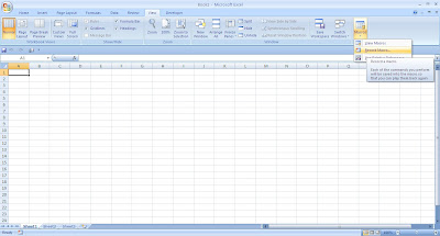
Then a new window opens with required specification like Macro name, Shortcut key, store macro in, Description
Note:
The Macro name should not conatin any blanks spaces or any special characters
For shortcut key, avoid usual shortcut keys like Ctrl+v, Ctrl+v etc.,
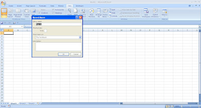
Once you clicked OK the macro start to record all your activities that you are doing in that excel. To stop the record, again go to views_> Macro-> Stop recording
View -> Macros -> Record Macro

Then a new window opens with required specification like Macro name, Shortcut key, store macro in, Description
Note:
The Macro name should not conatin any blanks spaces or any special characters
For shortcut key, avoid usual shortcut keys like Ctrl+v, Ctrl+v etc.,

Once you clicked OK the macro start to record all your activities that you are doing in that excel. To stop the record, again go to views_> Macro-> Stop recording
Introduction to Macro
When you find yourself repeatedly performing the same actions or tasks in your spreadsheets, it might be time for you to create a macro. A macro is a recording of each command and action you perform to complete a task. Then, whenever you need to carry out that task in your spreadsheets, you just run the macro instead.
Macros can be activate by a couple of keystrokes or by a worksheet button so they are easy to execute, and, provided they were recorded correctly, they will always carry out the same steps in the same order with no chance for operator error.
Although complex macros can be created in Excel using the Macro editor, it also possible to create relatively simple ones using the Excel macro recorder. If you are new to using macros in your spreadsheets, this is the right place for you to learn macros
Macros can be activate by a couple of keystrokes or by a worksheet button so they are easy to execute, and, provided they were recorded correctly, they will always carry out the same steps in the same order with no chance for operator error.
Although complex macros can be created in Excel using the Macro editor, it also possible to create relatively simple ones using the Excel macro recorder. If you are new to using macros in your spreadsheets, this is the right place for you to learn macros
Subscribe to:
Posts (Atom)